Building and calibrating a custom stereo sensor
We go through the process of building, synchronizing, and calibrating a custom stereo pair using Skip Robotics calibration tooling. Starting with two Blackfly S USB3 cameras, we add wide angle lenses, hardware trigger sync, and a high quality calibration to produce an accurate stereo sensor.
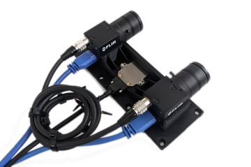
To test our calibration software, we're going back to basics and building a high-accuracy stereo camera from scratch. Of course, 'from scratch' is relative, and in this case we'll be using a pair of standard FLIR industrial cameras and CommonLands wide angle lenses (we are not affiliated with either company; other hardware would work just as well). We'll walk through the process of hardware selection, wiring, and finally calibration.
Sensor and Lens
The goal of our project is a high-accuracy stereo sensor, so we'll be using a grayscale global shutter camera module. Color sensors use a Bayer filter, reducing the effective resolution. Color images produced via Bayer filter have undergone an interpolation process which is not ideal for geometric computer vision applications. Similarly, a global shutter sensor is better for state estimation because we know each pixel was captured at the same moment in time. Luckily, high quality CMOS global shutter sensors are now available with many industrial camera modules!
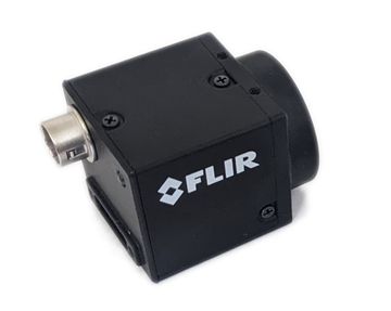
We'll be using two FLIR BFS-U3-16S2M-CS cameras, each containing an IMX273 1/2.3" global shutter sensor with a resolution of 1440 x 1080 pixels. These are USB cameras, which is not ideal for production robots (we generally recommend GMSL or GigE industrial cameras), but they work well enough for this project.
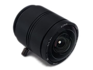
For the lens, we've picked the CIL032-F2.0-CSANIR from Commonlands. It has an approximately 90 degree horizontal field of view, good low-light performance at F/2.0, and relatively low distortion. If you don't need your sensor to work with IR illumination, you can opt for the IR cutoff filter version of the lens. In the past, we've also had good luck with lenses from Sunex Optics. In our experience, both companies provide good support and can help with lens selection.
Trigger Sync
A stereo sensor measures distances by comparing the position of objects in the left vs right camera, so it's important that the two images are captured at the same time. Otherwise, moving objects or a moving camera will distort our depth estimates. To get our sensors synchronized with minimal hardware, we'll connect them with a cable that allows one to trigger the other.
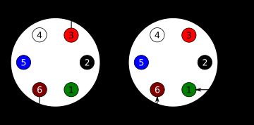
Teledyne FLIR provides a guide on how to trigger sync their cameras. In our design, we use the camera's non-isolated input pin, which doesn't require extra resistors in the cable. With this design we only need two wires connecting the cameras:
- The ground pins (pin 6) on both cameras must be connected to each other.
- Pin 3 (output line 2!) on the primary camera must be connected to pin 1 (input line 3!) on the secondary.
After physically connecting the two cameras, we need to configure them for trigger sync. We want each camera's image capture to start at the same time, but we also want the exposure time to match! To accomplish this, we'll configure the primary camera to control both the frame rate and and exposure of the secondary via a pulse transmitted through the cable.
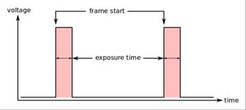
The exposure will start when the secondary's input line is activated and will end when it is deactivated. These settings can be configured using FLIR's SpinView tool.
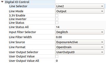
For the primary camera, we'll need to configure Line 2 for output. To do so, go to the 'Digital IO Control' tab, and pick 'Line 2' in the 'Line Selector' drop down. Set 'Line Mode' to 'Output' and 'Line Source' to 'Exposure Active'. This configures 'Line 2' to output logical high whenever a frame is being captured.
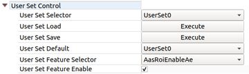
To make camera setting changes persistent, go to the 'User Set Control' and pick 'UserSet0' from the 'User Set Selector' drop down. Select 'UserSet0' from the 'User Set Default' drop down as well. Now click 'Execute' for the 'User Set Save' action. This will save the current settings as 'UserSet0' and make that the default configuration of the camera on start up.
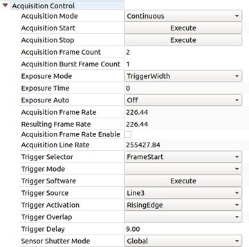
For the secondary camera, we'll need to go to the Acquisition tab and set 'Exposure Mode' to 'Trigger Width'. Note: It's normal for 'Trigger Mode' to be blank. We'll also need to set 'Trigger Source' to 'Line 3' and 'Trigger Activation' to 'Rising Edge'.
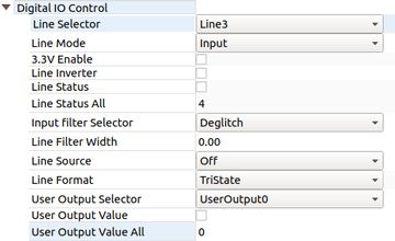
In the 'Ditial IO' tab for the secondary camera, we will select 'Line 3' as the 'Input Selector' and set 'Line Mode' to 'Input'. As with the primary camera, we'll go to the 'User Set Control' tab and save these changes to 'UserSet0' and make that the default User Set.
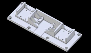
Mounting Bracket
An ideal sensor body for a stereo sensor should be very rigid; even very small amounts of movement between the two cameras will change the calibration. To illustrate this point, consider that a sensor with a horizontal resolution of 1,440 pixels and a 90 degree field of view has an average of 0.0625 degrees per pixel. If we're able to measure disparity down to a 0.1 pixels, our sensor will be sensitive to camera misalignments on the order of 0.006 degrees! Over a 10 cm stereo baseline, that corresponds to a deflection of ~0.01 millimeters! This level of stiffness is very difficult, if not impossible, to achieve. That said, we'll do our best with the materials we have.
Our stereo bracket design is 3D printed and will be mounted onto a metal optical stage which will provide most of the stiffness. We've also added some stiffening ribs to keep things as straight as possible.
Stereo Calibration
To calibrate our newly built stereo pair, we'll use the Skip Robotics camera calibration tool. We'll use a standard OpenCV rational polynomial lens distortion model and an AprilTag calibration target. Our camera calibration primer provides much more details about the target, data collection process, and math. Here we'll focus on the practical side of running the tool and validating results.
We'll start the Skip calibration tool using the following command:
$ skipr_calibrate_geometry -r 7 -c 11 -s 0.08 -t 0.05 --dataset flir_stereo_2023_05_09 --camera_file flir_stereo.json -i "stereo<desync_sec=0.001,skip_max=60>(aravis://FLIR-1E1001439F67-01439F67?fps=20&tare_clock,aravis://FLIR-1E10015FA3A4-015FA3A4?tare_clock)" --min_sharpness 0.05 --min_isotropy 0.6 --outlier_threshold 0.25 --target_warp --high_distortionCommand Line Parameters
Dissecting the components of the command line, we have several interesting pieces:
-r 7 -c 11configures the tool to expect a 7 by 11 calibration target.-s 0.08specifies that the checker board square size is 0.08 meters, or 8 cm.-t 0.05specifies that the AprilTag markers inside of each white square are 5cm.--datasettells the tool to store the calibration dataset in theflir_stereo_2023_05_09directory.--camera_filetells the tool to store the computed calibration data inflir_stereo.json.--min_isotropyand--min_sharpnessconfigure the acceptable blur level.--target_warpenables estimation of calibration target warping / bowing.--high_distortionenables a special mode for wide angle / high distortion lenses.-ispecifies the image sequence descriptor for recording the dataset.
An image sequence descriptor is a general purpose way for ingesting image data into Skip Robotics software. It consists of (possibly multiple) sequence URIs and commands for combining them. In the example above, the sequence descriptor is:
stereo<desync_sec=0.001,skip_max=60>(aravis://FLIR-1E1001439F67-01439F67?fps=20&tare_clock,aravis://FLIR-1E10015FA3A4-015FA3A4?tare_clock)This creates a stereo sequence by combining two monocular sequences. The stereo operator takes two arguments inside the angle brackets:
desync_secis the synchronization tolerance between left and right image timestamps.skip_maxis the maximum number of frames which can be skipped due to timestamp sync problems before the sequence fails. It also operates on two input sequences:aravis://FLIR-1E1001439F67-01439F67?fps=20&tare_clockaravis://FLIR-1E10015FA3A4-015FA3A4?tare_clock
The aravis:// prefix specifies the aravis input driver. These cameras do not support NTP time synchronization, so the image timestamps will be relative to camera start up. The tare_clock URI parameter estimates the offset between each camera's internal clock and the system clock prior to passing data to the stereo operator.
Using the Aravis driver, we can specify cameras using their internal unique id. In this case 1E1001439F67-01439F67 refers to the primary camera which will set the frame rate and control exposure time. We've configured the secondary camera to always follow the primary, so we do not give it a specific framerate in the sequence URI.
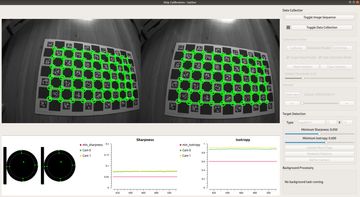
Data Collection
After starting the tool and turning on the camera stream, we'll see the screen below. We'll first adjust the lens on each camera to maximize the 'sharpness' value in the plot at the bottom of the screen. Once the cameras are focused, we can tighten the lens set screw (or glue the lens in place) and begin data collection.
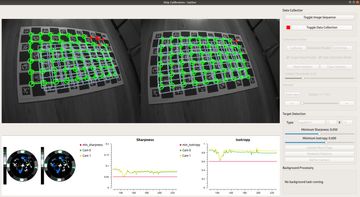
To capture the images needed for our calibration dataset, we'll hit the 'Toggle Data Collection' button and begin moving the camera in front of the target using the data collection path described in our calibration primer. The histogram display at the bottom left of the tool shows us the distribution of views we've collected in our dataset. The tool automatically rejects overexposed, blurry, and redundant images.
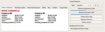
Calibration Results
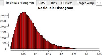
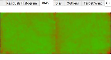
Once we're done gathering data, it's time to actually compute the calibration parameters. We do this by clicking the 'Calibrate' button on the tool and waiting ~30 seconds for the solver to run. When the solver finishes, our camera is calibrated and we can look at the reported statistics using the tabs at the bottom of the tool: