Calibrate Geometry Docs

Overview

The Skip Robotics intrinsic / stereo calibration tool is called CalibrateGeometry. It is an interactive GUI application for collecting data and estimating camera calibrations. The tool also includes functionality for inspecting and verifying calibration results.

Starting the tool

After installing, run the following command from the terminal to see the full list of arguments:

$ skipr_calibrate_geometry --help
version: 0.1.0
Program arguments:
  --help                                print usage help message
  -i [ --image_input ] arg              Source of images.
  -f [ --camera_file ] arg              The camera parameters file.
  --camera_fixed                        Camera fixed and target is being moved.
  -m [ --model ] arg (=RATIONAL)        The distortion model being used.
  -d [ --dataset ] arg                  The calibration dataset directory to
                                        use.
  --tag_family arg (=tag36h11)          The family of fiducial tags to look
                                        for.
  --tag_decimation arg (=2)             Detect fiducials tags using smaller
                                        image to improve speed. Image is
                                        reduced by this factor.
  -r [ --rows ] arg (=8)                The number of columns in the the
                                        calibration pattern.
  -c [ --cols ] arg (=6)                The number of rows in the calibration
                                        pattern.
  -s [ --square ] arg (=0.029999999999999999)
                                        The size of each chessboard square in
                                        meters.
  -t [ --tag ] arg (=0.024)             The size of each fiducial tag in
                                        meters.
  --min_control_points arg (=12)        The minimum number of control points in
                                        a calibration view.
  --min_sharpness arg (=0.10000000000000001)
                                        The minimum sharpness score to add
                                        calibration images to the dataset_.
  --min_isotropy arg (=0.84999999999999998)
                                        The minimum isotropy score to add
                                        calibration images to the dataset_.
  -n [ --max_images ] arg (=1000)       The maximum number of calibration
                                        pattern captures to use as part of the
                                        solution.
  --outlier_threshold arg (=2)          Threshold for removing outlier
                                        residuals. Measured in pixels.
  --target_warp                         Enable calibration target
                                        deformation/warp modeling.
  --high_distortion                     Enable solver mode for high distortion
                                        lenses.
  --residuals arg                       The residuals and auxillary solution
                                        data output file.

At minimum, the following command line arguments must be provided:

1. A image sequence / data source:

• --image_input

2. Parameters of the calibration target:

• --rows, --cols, and --square to specify calibration target geometry.
• --tag and --tag_family for AprilTag or Aruco target boards.

3. Locations where the collected dataset and output calibration will be saved:

• --camera_file for the calibration data output file.
• --dataset for the dataset directory.

For example, the follow command will start a calibration session for a UVC camera with an AprilTag based target. This assumes an 8x11 checkerboard pattern. Each square is 0.025m x 0.025m and the fiducial tags are 0.018m x 0.018m.

$ skipr_calibrate_geometry --rows 8 --cols 11 --square 0.025 --tag 0.01875 --image_input "uvc:///dev/video0" --dataset intrinsics_dataset -f calibration.json --tag_family tag36h11

GUI Overview

After starting the tool, you'll see the following screen:

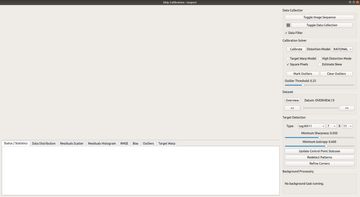
The GUI operates in two basic modes: data collection and data inspection. The initial screen shows an empty dataset in Inspect mode.

The right hand panel side shows various controls. The lower tabs show various reports about the dataset and calibration solution (when available). The upper left portion of the screen (blank in the screenshow above) shows the collected images.

Controls

The right hand side of the screen shows controls for data collection, running the calibration solver, viewing the images in the dataset, and calibration target detection.

Data Collection

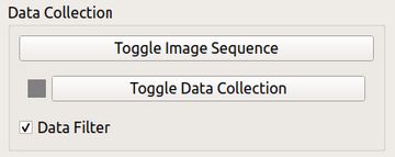
The data collection control panel is used for adding new images to the dataset from the image sequence source specified on the command line.

• 'Toggle Image Sequence' will start/stop reading images from the source.
• 'Toggle Data Collection' will begin actively collecting suitable calibration images.
• The 'Data Filter' checkbox enables filtering calibration images for quality / distinctness.

Calibration Solver

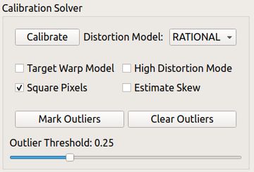
This is the main panel for running the calibration solver itself after collecting a dataset.

• 'Calibrate' runs the solver using the currently selected settings and saves the resulting calibration file to disk.
• 'Distortion Model' is used to select the distortion model used for calibration.
• 'Target Warp Model' models the calibration target as not perfectly planar, allowing better accuracy with imperfect targets.
• 'High Distortion Model' enables a special solver mode for high distortion lens. This is a slower, but more reliable algorithm when using lenses that have visually obvious distortions. It is recommended when straight lines look obviously curved in the camera image.
• 'Square Pixels' will constraint the x and y focal lengths to be identical. This is recommended for sensors with square pixels (most sensors).
• 'Estimate Skew' will estimate a skew coefficient in the intrinsics matrix. This is not necessary for most modern lenses and sensors.
• 'Outlier Threshold' controls the outlier rejection threshold (in pixels) for the solver. We recommend trying an initial value of '1 pixel' and adjusting as needed. The same threshold is used both for the robust cost function in the solver and for the outlier flagging button described below.
• 'Mark Outliers' will flag large outliers in the dataset so that they are not used by the solver. This button can be used to remove large outliers and rerun the solver for improved solution quality.
• 'Clear Outliers' will clear/reset all of the outlier flags.

Dataset

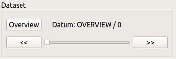
This panel is used to inspect the dataset and calibration results.

• When data is available, the slider will scroll through the collected images.
• The '<<' and '>>' buttons will advance forward and backward by a single image.
• 'Overview' will toggle to/from overview model. In overview mode, the inspection panel at the bottom of the screen will display aggregated statistics about the entire dataset. Otherwise, per-image data will be displayed.

Target Detection

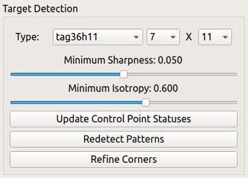
The target detection controls are used to configure the calibration target detector. This includes the type of target (classical, aptiltags, ChAruco, etc.) and the row x column dimensions of the checkerboard pattern.

• 'Minimum Sharpness' controls the sharpness / focus filter. Target detections which are too blurry will be skipped based on this threshold.
• 'Minimum Isotropy' filters detection with too much directional blur (motion blur). Values can range from 0 (no filtering) to 1 (blur must be perfectly isotropic). Values in the range [0.7, 0.9] are recommended for most applications.
• 'Update Control Point Statuses' will recompute the blurry / overexposure flags for individual corner points based on the current selected settings.
• 'Redetect Corners' will re-run the target detection algorithm on the current dataset from scratch. This is not normally necessary.
• 'Refine Corners' will rerun subpixel corner refinement only. This is not normally necessary.

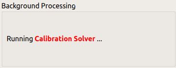
Background Processing

This area displays status text about long-running background operations, such as the solver.

Dataset collection and calibration

Starting from the initial screen, use the 'Data Collection' controls to start the image sequence. This will display a live camera feed in the upper left portion of the screen.

Align the calibration target in front of the camera and press 'Toggle Data Collection' to begin recording the dataset.

Once data collection is enabled, the tool with switch from 'Inspect' to 'Gather' mode:

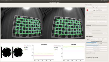
• A red recording icon will show up when recording is active.
• The top left portion of the screen will show the live camera feed with visualizations of the detected target.
• The bottom portion of the screen will display plots to help guide data collection.

Move the camera in front of the target slowly (or vice versa), collecting data from different angles.

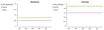
When a calibration target is detected, the average sharpness and isotropy of all detected corners will be plotted on the panel at the bottom of the screen.

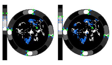
On the left of the sharpness plots, a histogram showing currently collected view angles and distances will appear. A separate histogram will appear for each camera in a stereo pair.

• Each histogram has a vertical bar on the left indicating the distribution of target-to-camera distance.
• The outer ring of the circular histogram on the right shows camera angles around the z-axis.
• The inner portion of the circular histogram on the right shows roll and pitch angles of the z-axis.

After collecting a dataset, press the 'Calibrate' button in the 'Calibration Solver' section of the control panel. This will run the calibration algorithm in the background.

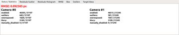
Dataset Statistics and RMSE value

When a calibration has been computed the tabs at the lower portion of the screen will show statistics and reports about the solution and dataset. In 'Overview' mode, these will be aggregated statistics over the whole dataset. Otherwise, the statistics will be reported on a per-image basis when you move through the dataset.

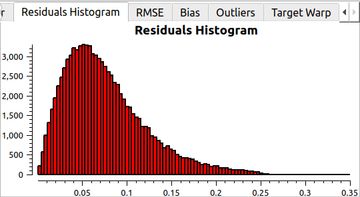
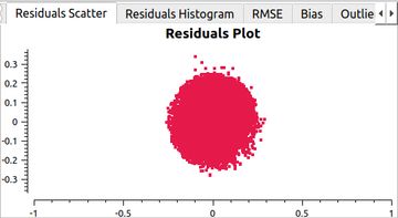
Residual Statistics

The 'Residual Histogram' and 'Residual Scatter' tabs show visualizations of the distribution of residuals. These can be used to confirm calibration quality.

Data Distribution

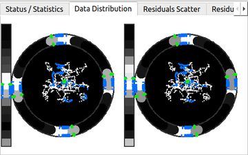
The 'Data Distribution' tab shows a histogram of the entire dataset, using the same format as the live histogram shown during data collection.

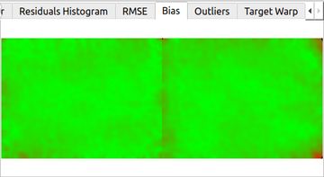
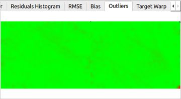
RMSE, Bias, and Outliers

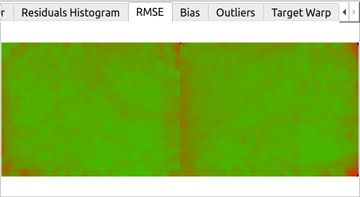
These tabs show a heatmap of the local RMSE error, bias, and the number of outliers. They can be used to confirm good data has been collected uniformly across the entire field of view and that there are not areas with poor data quality. Additional data can always be added to the dataset to fill in any gaps. The scale on these heat maps ranges from 0 to the scale of the outlier threshold set in the 'Calibration Solver' control panel.

Target Warp

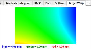
The 'Target Warp' tab shows the estimated physical target warping/bending as a heatmap. A legend at the bottom gives the numerical values in millimeters.