Repeatability of intrinsic calibration
If you calibrate a camera twice, will you get the same answer? It depends on how you calibrate. We collected 20 datasets to get to the bottom of things.
Summary
- If you use standard calibration tools, you have a risk of computing inconsistent, and often incorrect calibrations.
- In our experiments, the variations were up to 0.25 degrees on a 90 degree FOV lens. This corresponds to an error > 1cm at a distance of 3 meters and > 40cm at 100 meters.
- Collecting a large dataset of 300-500 images and verifying coverage across the entire field of view improves things, producing repeatability on the order of 0.01 degrees.
- The Skip camera calibration tool provides a reliable and convenient way to achieve this level of accuracy.
Why does it matter?
Many robots use cameras to perceive the world. To make use of the data, they need to detect objects of interest and find out where they are in 3d space. The 2d pixel location of a car isn't always enough to plan a path around it. We need calibrations to map from pixel locations to the real world.
The accuracy of camera calibration doesn't get a lot of attention. When it does, people speak in terms of RMSE error. Sometimes you will read 'RMSE is not a good indicator of accuracy', but this is usually as far as it goes.
In this article we'll dive deeper into what it means to have a good calibration. Instead of looking at just RMSE, or even the parameter values, we'll go to the basic physics and analyze the light ray vectors corresponding to each pixel. At the end of the day, this is what we need to get right.
What is repeatability?
Repeatability refers to the closeness of multiple versions of the same measurements. It quantifies the consistency of a process. Repeatability differs from accuracy in that it does not measure the difference from the true value of the thing being measured. That said, if our calibration process is not repeatable, we can't rely on it to run our robots.
What did we do?
We measured the consistency of repeated calibrations using different tools and data collection strategies. We collected 10 independent datasets using the built-in ROS camera calibration tool and 10 more using the Skip Robotics calibration tool. The camera was a 1440x1080 USB FLIR BlackflyS with a 90 degree field of view.
Methodology
Data was collected by moving the camera above a target placed on the floor. Photography lighting was used to provide good illumination of the target. A standard checkerboard pattern was mounted on an aluminum composite panel and used as the calibration target.
ROS calibration tool
We used the ROS camera calibration package and followed the process recommended by this tool. The python GUI was used to collect data, ensuring that the X, Y, Size, and Skew indicators turned green. The x and y focal lengths were constrained to be equal since almost all modern cameras have square pixels.
The following command line was used:
$ rosrun camera_calibration cameracalibrator.py --size 6x10 -k 6 --fix-aspect-ratio --square 0.08 image:=/camera/camera_0Following the ROS recommended procedure resulted in roughly 40 - 60 images per dataset.
Skip Robotics calibration tool
The Skip camera calibration tool was used for both data collection and as the solver. A more thorough data collection process was used as described in the Data Collection section of our camera calibration article. The x and y focal length were constrained to be equal and an outlier threshold value of 0.5 pixels was used.
Following the Skip Robotics data collection procedure resulted in roughly 300 - 600 images per dataset.
Analysis
After collecting the data and running each of the tools listed above, we were able to compute 20 different sets of calibration parameters. The raw values are listed in the appendix at the end of this article.
Analyzing the results, we saw that the Skip calibration tool gave much more consistent estimates for the focal length and principal point:
| calibration tool | stddev[f] | stddev[cx] | stddev[cy] |
|---|---|---|---|
| Skip | 0.36 pixels | 0.46 pixels | 0.20 pixels |
| ROS | 4.66 pixels | 3.90 pixels | 3.75 pixels |
If you look at the raw data in the appendix, you will notice the distortion parameter values are wildly inconsistent from run to run! So much so that we didn't bother computing the standard deviations. This is true for both the ROS and Skip calibration tools. It happens because the calibration model parameters are not unique! It is possible for two sets of values to produce the same physical calibration.
Incoming ray images
As we saw in the previous sections, the raw parameter values are not unique and so are not great for evaluating repeatability. We need a way to directly compare the actual calibrations. This can be done by thinking back to the optical meaning of what we're doing. No matter how we choose to break down the math, at the end of the day we're mapping incoming rays of light to pixels.
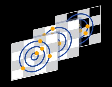
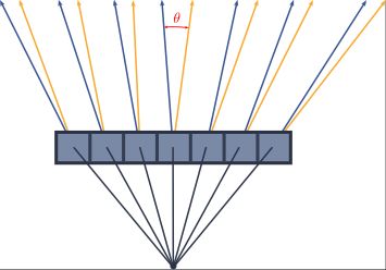
Instead of messing around with interpretations of model-specific parameters, we compared results using these rays. To do this, we inverted the calibration model by computing the incoming light ray direction corresponding to each pixel. While the parameters are not unique, the direction from which light will project on to each pixel is an actual physical quantity and is unique.
We form a 3 channel incoming ray image for each calibration by storing the unit vector / ray at each pixel location in the image. The angle between rays at corresponding pixels in different calibrations is a measure of similarity. We can use this to compare the repeatability of our calibration processes.
Rotational ambiguity
If you took a computer vision class, you may remember that intrinsic calibrations are not unique. It's possible to apply a rotation to the incoming light rays, and a corresponding inverse rotation to the calibration target poses without changing anything.
This makes it tricky to directly compare the incoming ray images. We accounted for this ambiguity by computing an optimal rotational alignment between the sets of incoming rays.
Measuring repeatability
For each pixel in the image and for each of the different approaches, we computed the average ray direction over the 10 datasets. We then measured the deviation relative to the average rays. The full procedure:
- Compute calibration parameters for each dataset
- Compute the incoming ray image for each dataset
- Rotationally align the incoming ray images
- Compute the average ray directions across all 10 datasets for each approach
- Compute the angular deviations of the incoming rays from this average.
Results
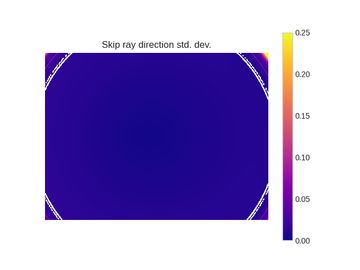
Following the methodology above gave us per-pixel measurements of repeatability for each of the approaches being evaluated. These are plotted below with brighter colors indicating higher variance and lower repeatability. The units for all of the plots in this section are degrees. Lower numbers are better and blue is the best.
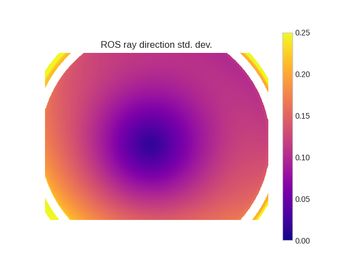
The repeatability is higher towards the center and increases as we go towards the edges. To better visualize the results, we aggregated the data as a function of distance from the center. The next set of plots show both the standard deviation and maximum deviation vs the distance from the image center (expressed as a fraction).
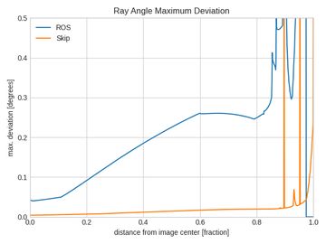
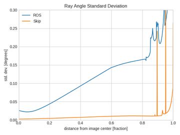
The latter set of plots show how much more consistent the Skip tool and procedure is compared to the ROS default. While we didn't directly measure accuracy with this experiment, we believe a proper evaluation of accuracy would produce similar results.
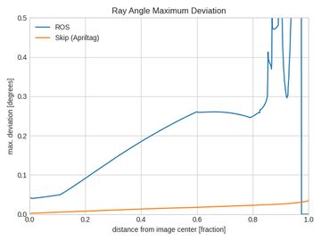
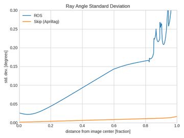
You may be wondering about the jagged spikes in the plots above. They're caused by failure of the numerical algorithm used to compute the incoming ray images. Using a traditional checkerboard caibration pattern makes it extremely difficult to get coverage at the edges and can cause the rational polynomial distortion function to behave poorly. We collected 10 more datasets with the Skip calibration tool using an Apriltag board to remove these artifacts. This substantially improved the results:
Conclusion
The plots shown above make it clear that your calibration method matters! Despite both solvers in theory optimizing the same function, the way you collect data and handle outliers is important. The Skip calibration tool results in a standard deviation of < 0.01 degrees (!!) almost all the way to the corners of the image. The ROS tool produces variations an order of magnitude higher, going over 0.20 degrees.
Looking at the maximum deviation, you can see that the ROS approach produces variations up to 0.50 degrees at the image edges! These sorts of errors may not matter for some applications, but if you're relying on your cameras for long range perception, safety, or visual SLAM, your downstream algorithms could be losing substantial accuracy and reliability.
Appendix: Solution Data
The following tables list the raw calibration outputs from the datasets collected above.
| dataset # | type | size | f | [cx, cy] | distortion |
|---|---|---|---|---|---|
| 1 | ROS | 41 | 926.80 | [705.88, 586.20] | [-0.391402, -0.151010, -0.001183, 0.000857, 0.060074, -0.071942, -0.362822, 0.086838] |
| 2 | ROS | 40 | 932.33 | [707.43, 582.87] | [ 2.083299, -2.393221, -0.000224, 0.000843, -0.485022, 2.409797, -1.832735, -1.317832] |
| 3 | ROS | 33 | 928.58 | [711.53, 586.24] | [ 5.407238, 45.577351, -0.000553, 0.000637, 7.387898, 5.702428, 47.402705, 20.854702] |
| 4 | ROS | 32 | 928.16 | [706.78, 586.15] | [ 7.419529, 96.743910, -0.000885, 0.000840, 17.030491, 7.711093, 99.304286, 46.014901] |
| 5 | ROS | 44 | 937.31 | [707.66, 582.05] | [ 0.125249, 7.049415, 0.000133, 0.000500, 1.670893, 0.454896, 6.972762, 4.020057] |
| 6 | ROS | 68 | 934.15 | [706.74, 579.89] | [-9.096051, 49.084826, -0.000004, 0.000634, 10.039802, -8.780796, 46.171620, 26.108922] |
| 7 | ROS | 56 | 935.72 | [711.03, 584.62] | [ 0.690867, 4.588634, 0.000450, 0.000815, 0.722842, 1.010778, 4.762238, 2.083320] |
| 8 | ROS | 51 | 929.04 | [709.79, 585.65] | [ 2.272459, -2.132392, -0.000644, 0.000875, -0.589066, 2.588201, -1.477768, -1.413566] |
| 9 | ROS | 57 | 934.03 | [704.05, 574.86] | [ 1.580550, -0.668105, -0.000104, 0.000171, -0.210967, 1.904577, -0.249565, -0.504082] |
| 10 | ROS | 60 | 922.20 | [698.05, 579.91] | [ 0.013453, -0.933862, -0.000498, 0.001318, -0.118444, 0.330385, -1.016716, -0.362605] |
| dataset # | type | size | f | [cx, cy] | distortion |
|---|---|---|---|---|---|
| 11 | Skip | 418 | 939.34 | [705.53, 574.03] | [202.311470, 75.495294, -0.000048, 0.000139, -1.759012, 202.738292, 139.965928, 6.049937] |
| 12 | Skip | 407 | 938.61 | [705.85, 574.69] | [ -0.329622, -0.431796, -0.000057, 0.000183, -0.016381, -0.010174, -0.620368, -0.089124] |
| 13 | Skip | 550 | 939.11 | [705.80, 574.39] | [ 30.071516, 7.833642, -0.000046, 0.000138, -0.808541, 30.402294, 17.325587, -0.648506] |
| 14 | Skip | 489 | 939.48 | [705.57, 574.59] | [ 1.024958, 0.058090, -0.000085, 0.000180, -0.023871, 1.345837, 0.298610, -0.045486] |
| 15 | Skip | 526 | 939.31 | [705.71, 574.52] | [ 1.714615, 0.934232, -0.000110, 0.000135, 0.055812, 2.033955, 1.402928, 0.238608] |
| 16 | Skip | 492 | 939.10 | [705.71, 574.64] | [ 0.430533, 0.119727, -0.000111, 0.000176, 0.022895, 0.750760, 0.173302, 0.061176] |
| 17 | Skip | 453 | 938.91 | [705.87, 574.67] | [122.781787, 35.887694, -0.000170, 0.000116, -2.886402, 123.135722, 75.027256, -1.289157] |
| 18 | Skip | 537 | 938.57 | [704.76, 574.64] | [ -0.401918, -0.238549, -0.000095, 0.000222, 0.017312, -0.082557, -0.448464, 0.006487] |
| 19 | Skip | 500 | 938.46 | [704.71, 574.46] | [ -0.336468, -0.138071, -0.000055, 0.000243, 0.024241, -0.017532, -0.324663, 0.035816] |
| 20 | Skip | 558 | 938.68 | [704.91, 574.55] | [ 0.728813, 0.067215, -0.000113, 0.000188, -0.003045, 1.049001, 0.214508, -0.001011] |