Fisheye camera calibration
We explain how to use fisheye lenses on your robot, focusing on EUCM projection.
Why use wide angle lenses?
Using high field of view lenses allows us to build robots with better sensor coverage using less hardware. It's vital for safety-critical designs capable of detecting hazards from all directions. Designing a robot that meets these specifications with narrow angle lenses requires twice as many cameras! Not only is this more expensive, it also increases bandwidth requirements, data storage, and overall system complexity.
What's the problem?
When you start using high field of view cameras, you will run into some challenges with your computer vision stack. Classic computer vision only works up to 180 degrees field of view. Depending on your lens, the problems may even start before that. You won't be able to calibrate and use wide angle cameras effectively without understanding camera projection models. In this article we'll provide an overview of the math needed to understand fish eye optics. We'll focus on the EUCM, which is the most popular and versatile wide angle projection model used in robotics. It is also the projection model we chose to implement in our camera calibration toolkit.
What is a projection model?
Most of computer vision assumes a pinhole camera with a distortion function to account for lens imperfections (see our camera calibration primer for more on distortion). This treatment gives a special place to the pinhole projection model as a natural ideal. In reality, the pinhole model is one of several projection functions, and is distinctly not ideal for wide angle lenses.
The projection and distortion models combine to map the incoming light rays to image pixels, so why do we need distortion? The difference is computational. The projection model is simple, fast, and invertible. This makes it directly usable in computationally heavy algorithms.
Distortion accounts for how the lens departs from this simple model. These corrections are applied once to each image as a preprocessing step. Afterwards, the more computationally efficient projection model can be used.
Projection functions
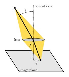
Now that we've covered some background, let's dig into the actual models. Lens projection models are typically characterized in terms of how incoming rays of light behave. Lenses have rotational symmetry, so projection models can be effectively described in terms of the angle between the optical axis and each incoming light ray. A lens projection curve captures the relationship between this angle and locations on the imaging plane.
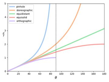
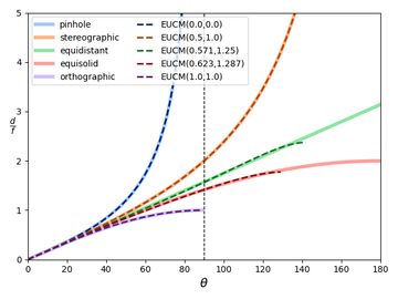
Fisheye lens manufacturers often use equidistant projection (explained below), but other commonly used projection models include equisolid, stereographic, and orthographic. The figure below show the projection curves for these commonly used models.
Pinhole projection: \( d = f\cdot\tan(\theta) \)
The pinhole camera model is the classic projection on to the \( z=1 \) plane. Each 3d point \( [x, y, z] \) is mapped to the 2d point \( \frac{[x,y]}{z} \). The model fails when z approaches 0 and is only valid up to 180 degrees field of view. The pinhole projection is the only one that always maps straight lines in object space map to straight lines in the image.
The downside of this model is substantial distortion at higher fields of view. The closer we get to the singularity at +-90 degrees, the more stretching we get. This makes it practically unusable for lenses with large fields of view.
The pinhole/rectilinear projection model is sometimes also referred to as the \( f\cdot\tan(\theta) \) model because the distance of a projected point from the image center is proportional to the tangent of the incoming ray angle.
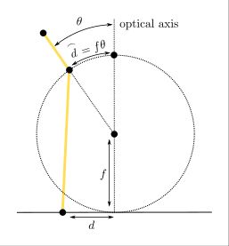
Equidistant projection: \( d = f\cdot\theta \)
With equidistant projection, the distance of a projected point from the image center is directly proportional to the incoming ray angle. This means there is no singularity at z=0, and lenses up to 360 degrees field of view can theoretically be represented. In practice, objects appear increasingly compressed as the field of view gets larger, although this effect is moderate even at high angles.
Equisolid projection: \( d=f \cdot 2 \sin(\frac{\theta}{2}) \)
The equisolid model makes sure that the area covered by each pixel is constant across the entire field of view. This model tends to compress image pixels excessively at large fields is not usable about ~190 degrees field of view.
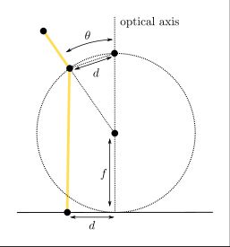
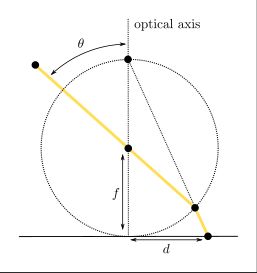
Stereographic projection: \( d = f \cdot 2 \tan(\frac{\theta}{2}) \)
This model first projects onto the surface of a unit sphere, followed by projecting the sphere's surface using pinhole projection. The stereographic projection model tends to represent object shapes accurately event at the limits of its field of view. Compression and stretching of image data is relatively limited, even at high ray angles. Lenses designed with this model are not common, but they do exist. The illustration below illustrates the projection geometry.
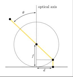
Orthographic projection: \( d = f \cdot \sin(\theta) \)
The orthographic model first maps on to a unit sphere, than perpendicularly down to the \(z=0\) plane, as illustrated below. This model is limited to 180 degree fields of view and compresses pixels to the point of being unusable well before this hard limit.
Enhanced unified camera model (EUCM)
The EUCM doesn't correspond to a specific physical lens geometry. In fact, it's actually a flexible family of projection functions with two parameters -- \( \alpha, \beta \).
It introduces a small change to the pinhole projection function. Instead of dividing by \( z \), we now divide by a normalizing function \( \eta(x, y, z) \). This turns out to be extremely powerful because it lets us model many different lens geometries with minimimal computational overhead.
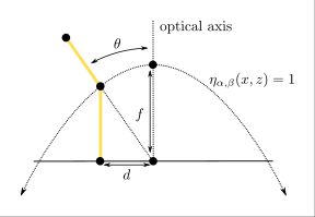
The normalizing function used by the EUCM is: \[ \eta_{\alpha, \beta}(x, y, z) = \alpha \sqrt{\beta(x^2 +y^2) + z^2} + (1 - \alpha)z \] Under the model, a 3d point \( [x, y, z] \) is mapped to \( \frac{[x, y]}{\eta(x, y, z)} \). When \( \alpha = 1 \) and \( \beta = 0 \), this reduces to pinhole projection. Other parameters generate different projection surfaces instead of the \(z=1\) plane.
When combined with a distortion model, EUCM can be used with many different lenses without having to know the exact optical design. The figure below show the EUCM parameter values which approximate the classical fish eye projections discussed above.
Picking the right model
It's important to pick the right projection and distortion models for your camera. The right choice depends on two factors: the optical design of the lens and its field of view.
For narrow angle cameras (< ~60 degrees field of view, or \( \theta < 30^\circ \) in the above plots), the differences between projection models are relatively small. We can often correct the non-pinhole projection via our distortion model, even if the lens isn't rectilinear.
As the field of view gets larger, the needed corrections begin causing too much pincushion distortion. For cameras with in the 60 - 120 degree range, the lens design becomes very important. Some lenses in this range are rectilinear despite having a very high field of view. In this case the pinhole projection model can be used with an appropriate distortion model.
More commonly, high field of view lenses are designed using the equidistant or equisolid model. In these cases we're forced to use a more complicated projection function such as the EUCM.
Our camera calibration tool supports both pinhole and EUCM projection, along with several different distortion functions. This lets you experiment to find the best combination for your use case.