Camera Calibration: A Primer
Camera calibration has been a mostly solved problem for decades. Why is it still painful? In this article we go into the practical difficulties that make production calibration trickier than it looks. We'll start with a review of the math and then share some practical tips for making it work well.
What is camera calibration and why do we need it?
Cameras are the sensor of choice for computer vision, and if we want to use them for any type of geometric application, they need to be calibrated. While deep learning has largely replaced classical computer vision for object detection, for many robotics applications we still need to map pixels in the image to physical geometry in the world. This task requires a calibrated image sensor.
Many robotics engineers have experienced the havoc caused by flaky calibrations. Algorithms breaking on one robot, but not another. Real bugs being written off as 'bad cal'. Bad calibrations causing good algorithms to look bad. It's an insidious dynamic that frustrates everyone downstream of the camera data and kills progress.
The goal of this article is to help engineers develop a camera calibration process that they can trust. We'll review some theory on how images are formed before getting into optimization and data collection. If you've ever been confused trying to match up the OpenCV calibration source code with it's documentation, this may be helpful! We'll focus on intrinsic calibration and leave extrinsics for another day.
The Pinhole Camera
One of the challenges with real world calibration is that the model taught to most people is the simplest one, but is not always applicable. That said, we'll start with a quick review of the traditional pinhole camera as motivation for a more general calibration model.
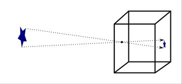
The pinhole camera is the original camera and the simplest device which can capture an image. It uses no lens or optics; just a box with a small hole punched through one side. The pinhole makes sure only one ray of light from each point in the scene enters the camera. Rays will travel from the object points, through the pinhole, and project onto the back surface of the box to form an image.
The model is simple, but it captures the essence of the imaging process and provides a mental framework for more sophisticated models. It's also convenient for computer vision because of it's many useful geometric properties. In the following sections we'll use the pinhole camera as a starting point to develop a practical model for camera calibration. Later, we'll discuss how different types of lenses alter the pinhole model and calibration process.
A Simple Image Formation Model
The image formation model describes how light from the scene is transformed to produce an image. We'll start with a simple model based on the pinhole camera with a sensor attached to the back interior wall, a distance \( d \) from the pinhole. The pinhole will be at the origin of our coordinate system, with the z axis pointing forward.
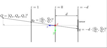
A point, \( Q \), in the scene will be projected to a point on the back wall of the camera. We can compute the coordinates of this projection on the \( z = -d \) plane: \[ q = -d \cdot [\frac{Q_x}{Q_z}, \frac{Q_y}{Q_z}]^t \] After light is projected onto this plane, it is registered by the sensor and converted into a discrete image.
The process can be broken down into two stages. First, we project onto a virtual projection plane at \( z = 1 \). This operation does not depend on any camera parameters other than the concept of pinhole projection. Second, we map from the virtual projection plane to image coordinates. This mapping captures the focal length and other parameters related the precise position and orientation of the sensor.
Going from projection plane coordinates to image coordinates involves two scaling factors. First, the image is scaled by the focal length to go from the virtual plane to the actual plane of the sensor. The second factor converts from metric coordinates to image coordinates based on the sensor's resolution. When calibrating a camera, we can only directly observe the image coordinates, and so we can only estimate the product of the two factors. This combined factor is commonly called the 'focal length' in computer vision applications, but it's measured in units of pixels.
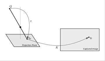
We'll call the projection operation \( \pi \) and use \( K \) (the camera transform/camera matrix) as the mapping from the virtual projection plane to image coordinates. For the pinhole camera model, these functions are defined as: \[ \begin{align} q_p =& \pi(Q) = [\frac{Q_x}{Q_z}, \frac{Q_y}{Q_z}]^t \\ q_i =& K(q_p) = \left[ \begin{array} ~f_x & 0 \\ ~0 & f_y \end{array} \right] q_p + \left[ \begin{array} ~c_x \\ ~c_y \end{array} \right] \end{align} \] The \( f_x, f_y \) variables above will subsume both the camera's focal length (distance of the sensor from the pinhole), and the resolution of the sensor. The \( c_x, c_y \) variables capture the offset of the image coordinate system from the projection plane.
The projection operation maps 3d points in the scene to points on a canonical projection plane. The camera transform captures the displacement, scale, and distance of the sensor relative to the optical axis, as well as the sensor resolution. This split may feel unmotivated, but it sets the stage for a more flexible model which can be used with many different lens types.
Lens Distortion
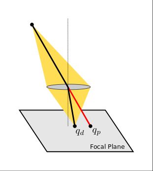
To make sure the image is in focus, the hole in a pinhole camera must be as small as possible. This limits the amount of light entering the camera and makes the physical pinhole camera more of a curiosity than a practical device. Lenses are used to overcome this limitation by capturing light from a wider area, but still focusing it on to a single point. They do this by ensuring all rays of light from a single point in the scene converge onto a single point on the image focal plane.
A lens increases the amount of light captured by each pixel, but it also bends the light and introduces distortions. These distortions are departures from the ideal pinhole camera projection function described in the previous section. While narrow field field of view lenses often approximate a pinhole camera, there are limitations to what is possible with lens design. As the angle of incoming light increases, most lenses depart from the pinhole camera model.
A distortion model can be used to compensate for these effects and other manufacturing variations. Instead of modeling the operation of a real lens, it is convenient to use the composition of a simple projection function with a distortion mapping.
The distortion function, \( D \), is a third component added to the image formation model between the projection and camera transform. This function is applied after an object point is projected on to the virtual projection plane. It maps from an ideal set of points on the projection plane to the real, observed image locations. Any one-to-one smooth transformation of the projection plane can be used as a distortion function. \[ D: \mathbb{R}^2 \rightarrow \mathbb{R}^2 \] By adding \( D \) we are modeling the entire camera as a simple pinhole projection, followed by a warping of the projection plane. This works well for many real world cameras, especially when more elaborate distortion models are used.
The breakdown of the image formation process into a projection, distortion, and camera transform is entirely artificial, so there is not a hard line between these steps. Theoretically, any distortion can be subsumed into a more elaborate projection model, and vice versa.
The Full Image Formation Model
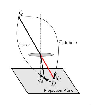
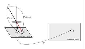
After adding distortion to the mix, we're ready to review the full image formation model. Combining projection, distortion, and the camera transform gives the follows steps to get from a scene point to the final captured image:
- projection \( \pi: Q \rightarrow q_p \)
- distortion \( D: q_p \rightarrow q_d \)
- camera transform \( K: q_d \rightarrow q_i \)
These are illustrated in the figure below. Note that \( q_p \) and \( q_d \) are in the projective plane \( \mathbb{P}^2 \) and correspond to 3d directions rather than 2d points. By using the \( z = 1 \) plane we are simply taking advantage of the fact that rays through the origin are in 1:1 correspondence with points on this plane.
Mathematically, the three steps above can be combined into one operation, but there are practical reasons to keep them separated. The projection model is meant to be a fast operation that can be computed efficiently as part of various algorithms. It can be applied to large numbers of points in fast, inner loops of code. The distortion function, on the other hand, is typically computed once to rectify each input image into a virtual image under an ideal projection. Separating the distortion and projection functions allows us to make use of the theoretical properties of pinhole projection geometry even when using real world lenses.
Rectification
Rectification is used to turn an image captured with lens distortions into a virtual image captured by an ideal pinhole camera. It's implemented as a remapping of image coordinate to 'undo' the distortions introduced by the lens. The rectification is performed once when each image is captured. Afterwards, we can work with an ideal, distortion free projection model. Rectification is the reason we split projection and distortion into separate functions.
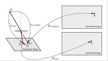
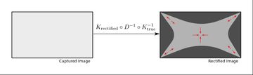
In the figure above, the rectified image represents a virtual image taken from an ideal pinhole lens with an arbitrary camera transform. The \( K_\text{rectified} \) camera transform can be kept the same as \( K_\text{true} \), or it can be altered to change the focal length, zoom, etc. We are free to pick \( \pi_\text{rectified} \) and \( K_\text{rectified} \) as needed for the application. The calibration process estimates \( \pi_\text{true} \), \( D \), and \( K_\text{true} \). In the end this gives us a coordinate transform which maps between the rectified image and the captured image. \[ q_i = K_\text{true} \circ D \circ K_\text{rectified}^{-1}(q_r) \] The above coordinate transform can be precomputed for every pixel in the rectified image to generate a coordinate table. We can use the coordinate table to efficiently generate a rectified image from each captured image. This enables us to get the best of both worlds by using mathematically convenient projection functions and complex lenses with the right optical properties for the application.
Wide Angle Lenses
The models described above are effective for narrow field of view lenses with relatively low distortion. Wide angle lenses have much stronger distortion when rectified to a pinhole model; this causes problems for the standard calibration approach.
The large amount of distortion causes inefficient use of the available image pixels. This compresses the image data at the center of the image, stretches the corners, and leaves gaps around the edges.
There are several strategies available for dealing with this problem. For moderate amounts of distortion typical of a 70 to 120 degree field of view lens it's often possible to rectify to a pinhole model anyway. This may mean cropping the rectified image to remove the hopelessly stretched corners and allow higher resolution at the image center.
Even with this compromise, initializing the calibration optimization problem for a wide angle lens can be tricky. Fitting high amounts of distortion requires a very flexible distortion function and convergence of the function parameters can require large amounts of data. One popular solution is to use a less flexible distortion model which can approximate a fisheye projection with very few parameters. This is the approach advocated by the ATAN/FOV model.
The pinhole model is fundamentally unsuitable for lenses approaching 180 degrees. The amount of distortion needed to rectify images becomes extreme, and the model simply breaks down at 180 degrees (intersection with the projection plane no longer exists). In this case we're forced to adjust the projection model itself. The Enhanced Unified Camera Model (EUCM) is a popular alternative projection model, but other options exist. A full discussion of projection models for wide angle lenses is enough material for its own post and will have to wait for another day.
The Calibration Process
With the image formation model out of the way, we can move on to the actual calibration process. To calibrate a camera, we need to know the relationship between points in the scene and where they end up in the observed images. To estimate this relationship for a particular camera, we need a dataset of scene points along with their corresponding image coordinates. We gather the dataset by capturing images of a calibration target from different angles and perspectives. The correspondences are thrown into a non-linear least squares estimator and a calibrated camera model comes out the other end.
In the follow sections we'll describe the calibration target, optimization algorithm, and the data collection process. Along the way we'll explain why collecting data and solving the optimization problem are more subtle than they seem. For high accuracy applications, a lot of care needs to be taken in both stages to get reliable results.
The Target
To gather data for calibration, we need a calibration target -- a rigid surface with a known pattern printed on it. The target has a set of identifiable control points on its surface which can be detected from the image. This gives us the needed correspondence between scene points and image points.
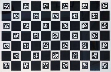
The most popular type of calibration target is a rigid board with a printed pattern. A checkerboard pattern is often used since it provides a grid of easily and precisely detectable corners. Other patterns used include circles and various custom patterns. More modern approaches use fiducial markers to uniquely identify the corners even if the entire pattern is not visible. This helps get observations at the image edges.
Calibration accuracy is limited by our ability to accurately manufacture a target with known dimensions and by our ability to detect the target's control points accurately in a camera image. The different patterns used vary in how difficult they are to detect and how accurately the control point location can be estimated.
Because real world lenses have a finite depth of field, it's important to make sure the target is in focus and at the target operating range for the application. This means it must be manufactured so that it covers at approximately 50% of the cameras field of view at this range. Using a smaller target closer to the camera will produce blurry images with poorly localized control points.
One of the sometimes overlooked sources of error in camera calibration is target manufacturing accuracy. It is surprisingly difficult to manufacture a large calibration target with control point positions accurate to within 1 mm. The most reliable solution for small scale targets is using a laser printer.
For large targets, a digital photo printer ("Digital C-print" or "Silver Halide Process") is the best choice. These printers use a laser or LEDs to expose photo paper and are the most accurate large format printer. Having a photo print shop professionally mount one of these gives a more accurate target than printing directly on the board.
Inkjet printers are commonly used, but large format inkjet printers can add several millimeters of error. For the highest possible manufacturing accuracy, lithography services can be used, but they are extremely expensive and unnecessary for most computer vision applications.
Once a target is printed, the next step is to mount it on to a flat, rigid surface. Here, again, scale becomes a problem. It is difficult to produce a large scale, flat, and relatively lightweight calibration target. Most surfaces will warp over time either due to storage, asymmetric water absorption, or the tension of the glue used to mount the pattern. We recommend using a reasonably rigid surface, and estimating the target's distortion as part of the calibration process. The Skip Robotics calibration tool has this functionality built in.
The Optimization Problem
A calibration is computed by optimizing the image formation model as a function of its parameters. This means each of the component function must be parameterized by a set of unknown variables written as subscripts: \( \pi_\alpha, D_\beta, K_\gamma \). The exact meaning of these variables will depend on the chosen model. We'll use the general purpose notation since it illustrates the concept.
To estimate the value of \( \alpha, \beta, \gamma \) we minimize a cost function based on the difference between the expected and observed image coordinates. Given a set of points in the scene \( \{Q_i\} \) and the corresponding observations in image coordinates \( \{q_i\} \), we want to minimize \[ \sum_i{||K_\gamma \circ D_\beta \circ \pi_\alpha(Q_i) - q_i||^2} \] as a function of \( \alpha, \beta, \gamma \).
Our problem is we don't know the locations of the points \( Q_i \) relative to the camera frame. The locations of the control points on the target are known, but we do not know the pose of the camera relative to the target. This means we have to add an unknown pose variable to our objective for each image captured. We'll call these poses \( \{T_j\} \) with each \( j \) corresponding to an image. \( T_j \) represents the pose of the camera relative to the target, or equivalently, the transform from the target's to the camera's coordinate frame.
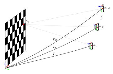
We're now ready to set up the full least squares objective for the optimization problem. We have:
- The set of known control points \( \{C_i\}_{i < N} \) in the target frame
- The transform, \( T_j \), from the target frame to the camera frame corresponding to the \( j^\text{th} \) image
- The image formation model \( K_\gamma \circ D_\beta \circ \pi_\alpha \)
- The image coordinates of the \( i^\text{th} \) control point detected in the \( j^\text{th} \) image; we'll call this \( o_{i,j} \)
The objective will minimize the squared distance between the expected and observed location of the control points in each image: \[ \sum_i{||K_\gamma \circ D_\beta \circ \pi_\alpha(T_j(C_i)) - o_{i,j}||^2} \] Our goal is to minimize this function with respect to \( \alpha, \beta, \gamma \) and \( \{T_j\} \).
The minimization itself is fairly straightforward using a non-linear least squares optimization library. As usual, though, the objective is not convex and will have local minima. Getting the optimization to converge to the right answer requires good quality data and a way to initialize all of the variables reasonably well.
Initialization
Before running the data and objective through an optimization algorithm, it's important to initialize the unknown variables to reasonable values. Starting the optimization at arbitrary values will almost certainly cause the solver to get stuck in a local minima. This is particularly true for the unknown pose variables.
The traditional way to initialize a calibration objective uses Zhang's algorithm. Zhang's algorithm makes use of the geometric properties of pinhole projection. Namely, it relies on the fact that pinhole projection of a planar calibration target can be described by a homography.
The algorithm computes a homography from each image of the target to the 2d target plane. The homographies are used to compute a closed form solution for the transforms \( \{T_i \} \) and the pinhole camera matrix \( K_\gamma \). Distortion is assumed to be minimal and ignored during this initialization phase.
Zhang's algorithm requires a pinhole camera model with distortions low enough that planar homographies are a reasonable approximation. This assumption is frequently violated by wide angle lenses, which require more sophisticated techniques beyond the scope of this article. The Skip Camera Calibration package, for example, uses an extra initialization phase for wide angle lenses to get around this problem.
Robustness
Despite our best efforts to collect good data, there will inevitably be some bad measurements. Robust loss functions make sure that the solution is not too heavily influenced by these one-off errors. This is done by adjusting the optimization algorithm to down-weight data points which have too much error. A full review of robust estimation is beyond the scope of this article, but any calibration solver should include robust loss functions and a method for removing gross outliers. Corners detected near over exposed areas of an image should also be removed.
Data Collection
Calibration data is collected by capturing images of the target from many different angles. For low volume calibration, the data can be collected manually by moving the target in front of the camera, or moving the camera in front of the target. For higher volume, a robotic arm can be used to gather data automatically as part of a production line. In this section we'll review best practices for gathering a good dataset. We will address observability, data balance, blur, and lighting requirements.
The concept of observability deals with how much information about the unknown parameters can be inferred from the data we collect. In many optimization problems, there are degenerate configurations of the data which don't provide enough information about the model. This happens when there are multiple sets of model parameters that explain our observations equally well.
With camera calibration there is ambiguity between the calibration target's distance from the camera and the focal length which cannot be resolved by frontoparallel images of the target. We need images in the dataset which capture control points with a wide range of camera frame z-values in order to observe the focal length. A good way to get this type of data is by holding the target at a 45 degrees tilt from the camera's optical axis. Higher angles tend to reduce accuracy because the foreshortening impacts our ability to precisely locate control point corners in the image.
The distortion function introduces two additional observability considerations. First, we need each target observation to span a large enough area to make the lens' distorting effects visible. We recommend having the calibration pattern span 25% to 50% of each image. Second, we need observation of the calibration pattern around the edges of the image. Lens distortion is typically minimal at the image center -- this is where most lenses behave like a pinhole camera.
Unfortunately, many calibration processes result in a majority of control points observed near the image center. Not having enough observations at the corners and edges gives poor calibrations that are hard to detect because the residuals look good! If the control point observations don't cover enough of the image edges, the calibration is likely to over fit towards the center of the field of view. This can be subtle for narrow field of view lenses since they stay close to the pinhole model, meaning a model fit at the center provides reasonable results at the edges. For wide angle lenses with a large amount of distortion at the edges, this type of image center bias will produce very poor results.
The number of control points observed in each image is also an important factor. Each captured image introduces an additional unknown pose variable with six new parameters (one for each degree of freedom). The image should increase the amount of information we have, so it must include enough data to both estimate the pose and contribute to our knowledge of the calibration parameters. A minimum of four control point observations are needed theoretically, but we recommend making sure there are at least 15-20 control point observations visible. It's important that these observations are not colinear, and ideally they should span a decent fraction of the image as mentioned above.
Observability is not a binary property. A single image of the target at 45 degrees is not enough to get a good estimate of focal length. Similarly, a dataset with 99% of the control points observed around the image center and 1% at the edges will not produce great results. This leads us to the idea of balanced data: a dataset needs a comparable number of observations from each angle, distance, and image region to avoid overfitting.
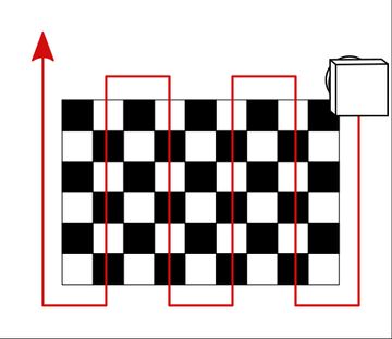
One strategy for a balanced dataset is to move the camera over the target with several passes of the pattern shown below. Start with a fronto parallel pass with the optical axis normal to the target. Follow with 4 more passes with a +-45 degree tilt around both the x and y axis. Each pass should include control point observations across the entire visual field from corner to corner and edge to edge. This approach can produce large datasets with hundreds or even thousands of images. A good sparse numerical solver can handle this amount of data on a laptop, with the optimization typically taking less than 30 seconds. The builtin OpenCV calibration routine will struggle with this much data and may run out of memory.
Up to now we've covered target positioning and data distribution, but have not addressed accuracy of individual control point observations. The main source of error here is sensor noise and various forms of blur. While blur caused by imperfect focus plays a role, the dominant source of error is typically motion blur. Relative motion between the target and camera during image capture will smear the corners and introduce substantial errors. Motion blur can be avoided by either avoiding fast motion (particularly rotations), or increasing the amount of light and reducing the exposure time. Using bright, diffuse lighting and the minimal practical exposure time is recommended.
Conclusion
We've gone over the basic theory of camera calibration and the considerations that should go in to building a robust camera calibration process. Along the way we've covered fundamental concepts like observability and practical advice on the 'black art' of collecting a good data. Many more pages could be written on any of these topics, but we hope this primer provides a good starting point and draws attention to the difficulties that are sometimes overlooked. It's easy to build a simple pipeline that can produce reasonable output, but it takes substantially more work to build a tool which provides consistent results in a production environment.
This article was born out of experience building our own calibration tool. We hope it helps you in your own journey to excellent and trouble free camera calibrations. If you have any questions, drop us a line via the contact page or just send an email to [email protected]; we're always happy to help!
References
- An Enhanced Unified Camera Model
- Straight Lines Have to be Straight
- Geometric Modeling and Calibration of Fisheye Lens Camera Systems
- Which Pattern? Biasing Aspects of Planar Calibration Patterns and Detection Methods
- Flexible Camera Calibration By Viewing a Plane From Unknown Orientations
- OpenCV Calibration Model
- Zhang's Camera Calibration Algorithm: In-Depth Tutorial and Implementation
- Multiple View Geometry in Computer Vision
- Accurate Camera Calibration using Iterative Refinement of Control Points